TURBULENCE MODELS AND ITS USE IN COMPUTATIONAL FLUID DYNAMICS (CFD)
Fluid dynamics is a basic branch of physics and engineering, it’s usage is huge and varies, starts from rocket and aircraft design up to biomedical fluid analysis. Although this discipline has long developed and widely used, its mathematical formulations in fluid mechanics are not solved yet, such as the Navier-stokes equation, a non-linear partial differential equation.
Unlike solid mechanic laws such as Newton’s second law, F = m.a, or kinetic energy E = 1/2.m.v2, the Navier-Stokes equation not always solvable with an exact method using available mathematical tools. Even, a special prize is prepared for whoever solves this equation (Millenium prize). One reason that this equation is unsolvable is the random, unsteady and unpredictable flow characteristics in certain conditions, or known as turbulence.
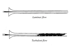
To be exact, turbulence is a fluid flow condition with a random and chaotic characteristic that contains eddy, swirl, and flow instability. And the opposite of turbulence is laminar flow, the flow with a predictable pattern and with no disruption in its paths. In laminar flow, the Navier-Stokes equation easily solved, for example, becomes a well-known equation Bernoulli equation (Navier-Stokes equation in steady-state and negligible viscous effect). Because of its complexity to solve turbulence flow mathematically, a well-known scientist, Richard Feynman said that “turbulence is the most important and unresolvable problem in classical physics”.

Because no analytical mathematics method could solve this problem, scientists try to quantify this problem based on the experiment. One of the most popular ones is the work of Osborn Reynold (1883), which found a non-dimensional ratio that could predict whether the flow is turbulent or laminar, and its called Reynold Number. Mathematically, Reynold number, Re is the ratio between internal force and external force, or Re = rhoVL/miu, with rho = density, V = velocity, L = characteristic length and miu = fluid viscosity. With this Reynold number, we could predict for example the flow trough a pipe is laminar if Re<2300, turbulence if Re>4000 and transition if 2300<Re<4000, regardless of what fluid we are using and the diameter of the pipe. This value states that if internal force is dominated than external force the flow will turbulent and vice versa.
Even though we can predict the occurrence of turbulence, but we cant model the flow specifically at any certain point in an arbitrary geometry. Instead of solving the Navier-Stokes equation to get the solution of turbulence in each “streamline paths”, scientists and engineers try to groups each turbulence eddies and solve those eddies as a single mathematical object. A lot of methods were developed based on this idea, such as averaging the flow parameter in each eddy or solve a certain size of an eddy, and proper selection of turbulence model is a big deal in Computational Fluid Dynamics (CFD).
Unfortunately, there’s no instant answer which turbulence model must be used to a certain problem, the answer really depends to the detail of the problem, even same problem will need a difference turbulence model, for example, calculation of the lift-and-drag coefficient of an aircraft will have different best turbulence model selection for calculation of wall shear stress in the same aircraft and flow condition. But, you don’t have to worry about this situation, because nowadays, a lot of scientists and engineers publish their research about CFD and share their turbulence model usage compared to the other which is best suitable for their detail cases as our reference to our cases. Nevertheless, this article will discuss some well-known turbulence models and the rule of thumb of its selection.
DNS (DIRECT NUMERICAL SOLUTION)
DNS is a method of directly solving the Navier-Stokes equation in the fluid flow without assuming the turbulence as an average flow parameter. Although ideal in terms of physical significance, this method needs huge computational as well as hardware demand and not feasible in common engineering cases.
LES (LARGE EDDY SIMULATION)
The turbulent flow consists of eddies with certain scales, sometimes it dominated with small or large eddies, ranging from kilometers to microns. LES modeling used to well-determined eddy scale, usually small eddy. This method also needs a huge computational effort but more reasonable compared to DNS.
RANS (REYNOLD-AVERAGE NAVIER-STOKES)
This model uses the average value of turbulence fluctuating parameters. This model is widely used in common industrial problems because of its low computational effort compared to LES or DNS even its accuracy is lower.
DES (DETACHED EDDY SIMULATION)
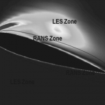
This turbulence model is the combination of LES and RANS, which solves near boundary layer region using RANS, and far boundary layer using LES. The picture below illustrates the DES concept.

In the region near boundary layer, velocity gradient becomes considerably high and determines the shear stress in the wall as well as turbulence boundary layer characteristics, to accommodate this situation, extremely small mesh must be used near the boundary layer, but this is sometimes not feasible in terms of computational effort and time, hence the wall-function is often used to modify velocity distribution in the boundary layer without considering extremely small mesh.
These are the commonly used turbulence models in the commercial as well as opensource CFD software and its rule of thumbs:
Spalart-Allmaras
- One equation
- No wall function
- Stable and easy to convergent
- Advantages: Aerodynamics flow and transonic regime
- Limitation : Not accurate for shear flow, separated flow and decaying turbulence
K-Epsilon
- Two equations
- Has wall function
- Easy to convergent and need relatively small memory
- Advantages: Free stream flow
- Limitation: Not accurate for no-slip wall, adverse pressure gradient, high curvature, and jet flow
K-Omega
- Two equations
- Omega is easier to solve than epsilon
- Has wall function
- Easy to convergent and need relatively small memory
- Advantages: Internal flow, high curvature, separation, and jet flow
K-Omega SST (SHEAR STRESS TRANSPORT)
- Two equations
- Has wall function
- Combination of k-epsilon for free stream flow and k-omega for near boundary layer flow
- Advantage: Separation and jet flow
- Limitation: Hard to convergence
LES Smargorinsky & Spalart-Allmaras
- Solves eddies flow in certain size/scale
- Separates small and large eddies
- Advantages: Thermal fatigue, vibration, buoyant flows
- Limitation: Hard to capture near-wall flow
To read other articles, click here.
aeroengineering.co.id is an online platform that provides engineering consulting with various solutions, from CAD drafting, animation, CFD, or FEA simulation which is the primary brand of CV. Markom.
Leave a Reply
Want to join the discussion?Feel free to contribute!